Feature engineering experiments 1: add log-returns-focused features

In this experiment, we test the impact of adding a returns-focused feature set (all quantities you can calculate for price, but for log-returns). This is a relatively small amount of work (applying the transformations you are already using to another variable). Just be sure they’re sensible in this context – a log-return is a two-point quantity (expressing a difference between two moments), whereas a price is a one-point quantity (exists at any given moment in time). For instance, it makes sense to apply moving averages, RSI, MACD, Bollinger (and many other TA indicators) to log-returns, but maybe some other indicators relying on e.g. volume information or open-close data do not.

The way we should go about these is to perform an A/B test, i.e.:

  • use your own default model;
  • record its performance across a set of (sufficiently long) time intervals (more than one to achieve statistical significance);
  • develop one of the above modifications;
  • add this to your own model;
  • record the performance of the modified model across the same set of (sufficiently long) time intervals;
  • quantify any differences and compare statistical significance.

We can collectively define some of the unknowns in the above plan (e.g. which time intervals, how long, which metrics) and I suggest you just propose what you’d like to use.

We invite Allora Forge participants and model builders to participate in this experiment!

The coordination of all feature engineering experiments takes place in this thread. The thread here is intended for ongoing work and results on the returns-focused feature variables.

4 Likes

Although I haven’t yet evaluated the impact of individual log-return-derived features on the model, the following is a report on how applying a selected set of these features improves performance. I will continue this analysis and provide a detailed report on the effect of individual features soon.

I planned my research process as follows:
I downloaded two full years (730 days) of ETH price data from Tiingo at 5-minute intervals and modified the dataset as described here. The data was then split into two parts—validation and test sets—ensuring that each contained sufficient context for training.

I began by fitting a linear regression model using varying look-back windows—our “context lengths”—to identify the optimal amount of historical data for forecasting. Treating context length L as a hyperparameter, I evaluated each candidate value on the validation set. For a given L, the model was retrained on the most recent L observations and then used to predict the next batch of returns. Each batch comprised 288 consecutive five-minute bars (one trading day), after which the window advanced by 288 points and the process repeated. This moving-window scheme ensured that the model continuously learned from fresh data while allowing us to empirically select the context length that maximized out-of-sample performance.

I believe that this walk-forward approach to retraining—rather than training on a fixed dataset and making all subsequent predictions—enables the model to continually adapt to new and emerging patterns. This is particularly important when working with time-series data, where market behavior can shift over time.

To determine the optimal context length, the model was retrained at each step using varying context sizes just before the test data. Three evaluation metrics were calculated across all batches (~6 months of validation data, totaling 50,000 prediction points) for each context length: directional accuracy (DA), relative absolute return-weighted RMSE improvement, and Z-transformed power tanh absolute error (ZPTAE). The results are as follows:


The optimal context length identified from this analysis was 20,000 (approximately 70 days), which yielded a directional accuracy (DA) of ~54.4%, a ZPTAE of 1.25, and a relative absolute return-weighted RMSE improvement of -25%.

Following this, I incorporated several log-return-based features into the dataset, including:

  • Bollinger Bands: Upper and lower bands derived from the rolling mean and standard deviation of returns over a 48-hour window.
  • Relative Strength Index (RSI): Calculated over 6-hour and 24-hour windows.
  • Moving Average Convergence Divergence (MACD): Computed using default parameters from Python’s TA package.
  • KST (Know Sure Thing): Also calculated with the default settings from Python’s TA package.
  • Simple and Exponential Moving Averages (SMA & EMA): Derived from the return series over 6h, 12h, 24h, 48h, and 96h windows to capture various trend horizons.
  • SMA Differences: Such as SMA(12h) − SMA(6h) and SMA(24h) − SMA(12h), to highlight momentum shifts.
  • Exponentially Weighted Standard Deviation: Computed using smoothing factors α = 0.01 and 0.05.
  • Trend Deviation: Defined as the difference between the 24-hour EMA of return and the current return.

Upon reevaluation with these features, the model’s directional accuracy improved noticeably across nearly all context lengths, while the relative RMSE improvement and ZPTAE loss remained largely unchanged.

It can be interpreted from the above plots that, when we extend the context window, both relative RMSE improvement and our custom ZPTAE metric rise steadily and then level off around the optimal look-back length, but DA doesn’t follow that pattern, and even declines with longer horizons. This suggests that DA on its own can be misleading, as you might correctly predict direction less than half the time yet still profit if your correct calls coincide with large market moves, a nuance that ZPTAE captures by scaling errors with volatility and return size. The drop in DA beyond the ideal window may also hint at overfitting to outdated patterns, whereas RMSE-based measures remain stable. Overall, this highlights the value of error metrics that weight by return magnitude, rather than relying solely on raw hit rates—especially when the model or its features aren’t yet strong enough to consistently make high-confidence directional predictions.

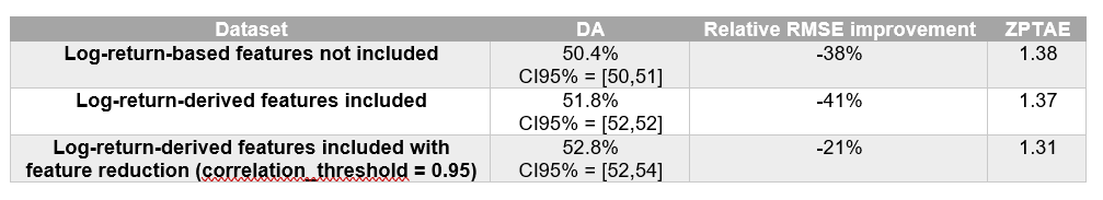
I then evaluated the model on the test set using three versions of the dataset: one without return-derived features, one with them, and one with return-derived features after applying feature reduction. The results below reflect the model’s performance when predicting log-returns over one year of test data—approximately 100,000 predictions—using a context length of 20,000 data points:

These results demonstrate that log-return-derived features significantly enhance the model’s performance, with feature reduction offering further improvements.

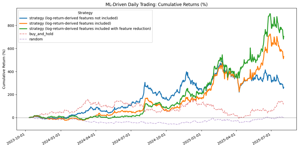
Finally, I trained the model on these datasets and simulated daily trading over a 2-year period, resulting in a total of 663 trades. The cumulative returns were as follows:

  • 260% for the model without log-return-derived features,
  • 530% with log-return-derived features, and
  • 708% with log-return-derived features plus feature reduction.

For comparison, simply holding the asset yielded a return of 122%, while random trading resulted in a -1% return. These results demonstrate the promising potential of log-return-derived features in enhancing model performance and trading outcomes.

5 Likes

I’ve put together a two-year ETH OHLCV dataset (5-minute intervals, from Tiingo) that we could all use as a shared benchmark for testing our models.

It covers 2023-08-142025-08-13 and is already split chronologically:

  • Train/Validation: 2023-08-152024-08-12 (~1 year)

  • Test: 2024-08-122025-08-12 (~1 year)

Both parts include log_return and target_log_return for daily return prediction. The split is designed to avoid data leakage and reflect the real-world case where we predict the future from the past.

Why this matters:

  • Consistent methodology – Everyone benchmarks models on the same dataset and time split.

  • Fair comparisons – Eliminates variability from random sampling.

  • Realism – Chronological split mirrors actual trading conditions.

How to load the dataset:

import pandas as pd
df = pd.read_csv(‘dataset.csv’, index_col=‘datetime’, parse_dates=True)

The idea:

  • Use this dataset (or similar ones) as a common benchmark.

  • Stick to consistent evaluation metrics.

  • Share results and approaches so we can actually learn from each other’s work instead of guessing why numbers are different.

Note 1:
Accuracy should always be reported on the test set.

Note 2:
If you’re using a rolling-window approach for training and testing, insert a gap of 288 data points (equivalent to 1 day) between the train and test segments. This buffer helps prevent data leakage by ensuring that no information from the test period leaks into model training.

2 Likes

I applied TA on log-returns ETH 24h LR

gML! I was curious what would happen if I took all the TA stuff I usually throw at price - RSI, MACD, Bollinger, ATR and instead applied it directly to log-returns. Would it help, or just add noise? So I set up an A/B test on ETH 1-day log-return and here’s what I saw.


TL;DR

  • 360 days of ETH 5-min OHLCV from Tiingo, horizon = 288 (24h).
  • Baseline: TA on price.
  • Variant: same TA but applied to 1-step log-returns r1.
  • CV: expanding folds with 24h embargo.
  • Metric: ZPTAE (σ from 100 non-overlapping daily returns).
  • Result: mean ZPTAE dropped from 0.5797 → 0.5610 (~–3.2%).
  • DM test: t=2.317, p=0.0205 → statistically significant.
  • Directional accuracy still ~51% (24h is hard), but stability improved.

1. Data & target

  • Source: 360 days of ETH 5-min OHLCV from Tiingo.
  • Target: y = log(close_{t+288}) − log(close_t).

I went with ZPTAE normalized by σ from 100 non-overlapping daily returns. With a 24h horizon, scale drifts a lot, so this made the loss feel more stable.


2. Features

Baseline (price-focused): EMAs/SMA, RSI, MACD, Bollinger bands, ATR & realized vol, plus calendar effects (hour, weekday, weekend).

Returns-focused (the new bit):

  • Lags of r1
  • Rolling stats: mean, EMA, std, sum, |r| mean, r² mean, skew, kurtosis
  • RSI, MACD, Bollinger on r1
  • “Returns energy/force”: rolling r1², Δr1

I skipped volume or open/close-based features since they don’t make much sense for returns.


3. Cross-validation

Expanding CV with three folds, each with a 24h embargo before test. I wanted to be extra careful not to leak.


4. Results

Model RMSE MAE Corr DirAcc ZPTAE
Baseline (price) 0.0441 0.0328 0.053 0.515 0.5797
Returns-focused 0.0433 0.0317 0.035 0.512 0.5610

DM test on ZPTAE said the difference wasn’t just noise.


5. What the charts told me

Figure 1 — Rolling ZPTAE (EWMA-100)

=> The orange line (returns) sits a bit lower than the blue baseline in many spots, especially during volatile patches. That gave me some confidence this is real.

Figure 2a — Prediction vs Truth (returns-focused)

Figure 2b — Prediction vs Truth (baseline)

=> Shapes are similar, but returns-focused scatters hug zero a bit tighter. Explains why corr didn’t move much but ZPTAE improved

Figure 3 — Residuals

=> Residuals are fat-tailed, as expected. Returns-focused tightens the center a little, which matches the lower ZPTAE.

Figure 4 — Timeline (returns-focused)

=> On big swings, my preds stay too flat. I sacrificed amplitude for variance control.

Figure 5 — Feature importance (Baseline)

=> Price model leaned on EMAs/SMAs and calendar stuff (weekend effect stood out).

Figure 6 — Feature importance (Returns)

=> With returns features, new ones show up: r_ma_144, bb_width_r_144, r_skew_288, r_kurt_288. The model is actually picking up on returns shape, not just levels.


6. What I learned

  • Just mirroring TA onto returns gave me a small but real gain.
  • The juice came from higher-moment and clustering features (skew, kurt, band width), not just lags.
  • Conservative preds = more stability. That’s good if you care about regret-style losses, but it means you under-react on big moves.

7. Next steps

  • Run ablations: check exactly which returns features drive the gain.
  • Try different σ definitions to see if the improvement holds.
  • Layer in multi-resolution returns (5m/15m/1h).
  • Maybe cross-asset returns (BTC, SOL) as extra context.
  • And I want to try a light calibrator to boost amplitude without wrecking stability.

Closing

I went in not sure if “RSI on returns” was going to be useful. Turns out, it’s not magic, but it does shave off loss and shows up in significance tests. Feels like a small but honest step forward.
Curious if anyone else sees the same thing or if you’ve tried skew/kurt features on returns and found them useful in different horizons.
Big thanks to @Apollo11 and the team for nudging me into the returns-focused path.
This little experiment already gave me something real to think about, and I’m planning to run a few more trials (ablations, different σ definitions, maybe cross-asset returns SOL-BTC-ETH x PAXG x USDT) to see how far this approach can go.

4 Likes

Really nice work @t-hossein. Thanks for sharing so much detail on your methodology. It really helps to understand and interpret the results.

I have a question about the moving-window setup and general data splits you were using. Since your prediction horizon is 24 hours and many of the engineered features (e.g. RSI, skew/kurtosis, Bollinger widths) use rolling lookbacks of up to ~1 day, there’s a subtle risk of data leakage at the train/validation boundaries if a purge gap isn’t applied inside each fold.

Firstly, because a data point from 24h in the future is needed to calculate the log return, there is a danger that there is label overlap between the training and test/val datasets. (This is a general difference of using [log] returns vs price to watch out for.)

Secondly, there can be feature overlap if the test/val datasets need rolling data from the training period.

To avoid this, the usual approach is to apply a purge gap ≥ max(prediction horizon, longest lookback) inside every walk-forward fold, i.e., probably a gap of at least 1 day, possibly 2 if any features look back further.

I wasn’t sure from your description whether you’ve already accounted for this in your moving-window CV. If you have, great. It’d be useful to confirm so others can align. If not, it might be worth re-running with a purge gap, since it can shift metrics like ZPTAE and directional accuracy.

3 Likes

@t-hossein great idea to create a common dataset which everyone can use to help compare model results!

2 Likes

@its_theday your work is impressively thorough, especially backing up the ZPTAE improvement with a DM test. That gives a lot of weight to the result and is something I’d encourage everyone to do.

I’d be very interested to hear how the ablation tests went. Were you able to rank features or groups of features (lags-only, bandwidth-only, shape-only) by delta ZPTAE?

Cool to see potential signal in the higher-order statistical moments. Since skewness and kurtosis generally need more data to estimate robustly, I’m curious if you see their feature importance increasing as the training size grows across your expanding folds? Or does their contribution stay roughly constant?

[Oh, and similar to my previous post, just checking that the 24h embargo is longer than the rolling lookback time, i.e., embargo ≥ max(horizon, lookback)].

2 Likes

@t-hossein @its_theday I really like how the two windowing approaches complement each other. Moving windows are great for testing adaptation and responsiveness to changing market conditions. Expanding windows are better for testing durability and stability over longer periods.

I wonder if there’s a potential hybrid approach? Use the expanding windows to learn how much history is needed to get a robust signal from features like skewness and kurtosis (since higher-order moments need more data to stabilise). Feed that insight into the moving-window scheme to improve responsiveness while still leveraging the shape-based features effectively. It’d be interesting to see if this could boost DA around volatility spikes and trend reversals, where responsiveness really matters.

2 Likes

Hey Steve, thanks a lot for the detailed suggestions!

Since I’m only using past data from the test batch, I don’t think rolling features would cause data leakage. Correct me if I’m wrong, but I think that issue would only arise if I included data that comes after the test batch.

As for the log-returns in the training data right before the test batch, that could indeed cause leakage in this setup. I’ve avoided this by inserting a gap between the training batch and the test batch. So, to be more precise, the scheme should actually look like this: