Thorough testing of new forecaster model

[joel]

Forecasting is the component that enables context-awareness in the Allora Network. During inference synthesis, worker inferences are combined using their historical performance (through an exponential moving average of their regrets) which can only take into account shifts in worker performance in future epochs. The role of forecasters is to use the current conditions to predict the performance of inference workers before the outcome is known. As such, the standard forecaster model should be able to identify outperforming inference workers and the situations in which they outperform, and improve upon the naive network inference.

A broad overview of the forecaster model was previously discussed here. This post details recent work on improving the standard forecaster model. We will discuss potential changes to the model structure, choice of target variable, feature engineering and testing/benchmarking with synthetic and real data.

[Apollo11]

Thank you for making this thread @joel!

Accurate forecasting is critical for Allora’s performance and I’m really looking forward to reading about your findings here.

[joel]

We first identified a number of potential improvements to the forecaster model.

Model structure: The first version of the forecaster made use of a global model, where inferer addresses were used as a categorical feature in training. However, if the forecaster cannot adequately distinguish information from different inferers with the address feature, then a global model may simply predict the mean for all inferers. As an alternative we consider a per-inferer method, with separate forecasting models for each inferer.

Target variable: As discussed in the Allora Whitepaper, the first model forecasts the losses for each inferer, which are then converted to regrets to be passed to the weighting function. A potential drawback of this method is that the loss-to-regret conversion must use the network loss at the previous epoch (i.e. R_forecast = log L_network,prev - log L_forecast) rather than the actual network regret (which is not yet available). If the network regret changes significantly from epoch-to-epoch this affect the final weighting. However, a benefit of forecasting losses is that they are independent for each inferer, and therefore do not depend on the makeup of the active set of inferers (see details about merit-based sortition here).

As alternatives, we consider models that instead forecast the regret or z-score of the regret for each inferer. This way, the forecaster only needs to predict the relative accuracy for each inferer, rather than the absolute accuracy (as for losses). However, these methods could then be sensitive to changes in the active set of inferers if the network loss changes significantly.

Feature engineering: A number of engineered properties (exponential moving averages and standard deviations, rolling means, gradients) require an epoch span to be defined for the calculation. As the optimal span length or combination of spans is not obvious (e.g. shorter or longer spans), we will test the combinations that produce the best outcomes. We will also test if the current features are sufficient to detect periodic outperformance, or whether further feature engineering is required.

Next, we must decide on a series of tests to identify the best performing model and feature set.

[joel]

We start with a simple, controlled test with a worker that follows sinusoidal outperformance in regret, aiming to test the sensitivity of features to periodic variables. In this test the sine function has an amplitude of 1, period of 10 and random error from 0-1 is added at each step. These figures show the true and predicted regret from a global model forecaster that predicts raw regret, and the relative importance of the top 20 features in the model.
The forecaster model picks up this periodic outperformance well, even with randomness of similar order to the sine amplitude, mainly through the rolling mean and difference from the moving average.

The next step is to increase the complexity of the test by adding another sinusoidal outperformer with a different period (17 epochs) and amplitude (1.5), along with other inferers that have random performance as a control. Here we can see that the regrets for the outperforming workers are being predicted independently, and inferer ID has become the most important feature.

In this case a per-inferer model might perform better than a global model, so we compare the predicted versus true regrets for the global and per-inferer models. Each set of coloured points in the figures indicate a different inferer (blue for the inferer with an amplitude, orange for the inferer with an amplitude of 1.5, the rest predict random values from -1 to 1), with the unfilled squares showing the medians and dashed lines showing linear fits. The black dashed line indicates a perfect 1:1 correlation.
As indicated in the figures, the per-inferer model is marginally better than the global model according to the root mean square error (RMSE), though not the mean absolute error (MAE). However, this is perhaps due to the larger scatter in the random inferers in the per-inferer model. If we only consider the sinusoidal inferers then the per-infer model outperforms in both metrics. This can be seen in the linear fits for the sinusoidal inferers, with the per-inferer model having fits closer to the 1:1 line, particularly the amplitude=1.5 worker (orange points). I.e. the per-inferer model is better able to distinguish performance of the two sinusoidal workers.

Global model:

Per-inferer model:

[joel]

Expanding on the sinusoidal periodic benchmark, we now test a benchmark where a worker outperforms for 1 epoch at regularly-spaced intervals, and otherwise shows random performance. This tests the sensitivity of the forecaster to non-continuous periodic variables. We first test a single worker with random regrets from -0.5 to 0.5, where the regret is increased by 1 every 10 epochs. The standard forecaster performs poorly on this test, failing to identify the outperformance epochs. Using EMAs/rolling means with combinations of different span lengths did not improve the performance of the model.

A simple solution to the problem is to add autocorrelation as part of feature engineering. In this case, regret with a lag of 10 epochs becomes the dominant feature, allowing the forecaster to ‘flag’ upcoming epochs of outperformance. The forecaster predicts a regret of ~1 in the outperformance periods and ~0 at other epochs, i.e. the mean in each case. This is the optimal strategy for this benchmark given the absence of any other contextual information (by design).

In practice we use both an autocorrelation function (ACF) and partial autocorrelation function (PACF) during feature engineering, and only select lags that are significant in both (>95% confidence). The PACF is used to remove multiples of shorter lags (i.e. 20, 30, 40, etc. in the above tests), but it can sometimes identify lags that were not found in the standard ACF.

[joel]

As a more realistic test, we create an experiment which uses geometric brownian motion (GBM) to generate ‘true market values’, with randomly modulated periods of drift. We then create inferers which outperform in different circumstances (uptrends, downtrends, crabbing), along with control inferers which predict random returns. This benchmark tests the ability of forecaster models to distinguish workers and connect outperformance with variations in the ground truth. In the test we start with an initial value of 1000 and volatility of 0.01. The drift parameter is randomly modulated between -0.01, 0 and 0.01 (downward drift, no drift and upward drift) for periods with a typical length of 5 epochs (with each period length drawn from a Poisson distribution). For the test we generate 2000 epochs of data, with 1900 used for training and 100 used for testing.
This figure highlights the drift periods in data generated for forecaster testing, with downward drifts shaded blue and upward drifts shaded red.

We start by comparing the inferences and regrets for the three outperforming workers, along with the predictions for a forecaster predicting raw regrets. These workers generate returns with an uncertainty drawn from a Gaussian distribution. The standard deviation for each worker is randomly drawn between 0.001-0.003 for accurate periods and between 0.005-0.01 for inaccurate periods. The other “random” workers draw standard deviations between 0.002-0.012.

The “downtrending” worker has three accurate periods beginning at blocks 1906, 1930 and 1947. The forecaster reasonably identifies each outperformance period where the worker’s regret increases to >0, with the predicted regret increasing from ~ -1 (during inaccurate periods) to ~0.5 (accurate periods).

The “uptrending” worker has two accurate periods beginning at blocks 1914 and 1984. The predictions from the forecaster have a similar behaviour to those for the downtrending worker.

The “crabbing” worker is accurate during periods of no drift. The true regrets for this worker have a more subtle behaviour, with the regret during accurate periods often barely increasing from the typical value of ~ -0.2 during inaccurate periods. This is because the “random” workers perform better during low drift periods, competing with the crabbing worker. Still, the forecaster is able to identify some periods where the crabbing worker will outperform, such as at blocks > 1992.

Putting it all together, we can use the mean log loss over the testing period to determine if the forecast-implied inference has improved upon naive network inference. In this test, the forecast-implied inference from the standard inferer (log loss=1.078) beats both the naive network inference (log loss=1.620) and the best worker in the network (log loss=1.641).

[Apollo11]

This is extremely rich @joel, thank you!

I love how you’re building up from simple periodic outperformance to more contextual periods of outperformance.

If I liberally translate, are you saying that forecasters should be able to identify which models outperform based on market conditions (bull/bear/consolidation)?

That would be very powerful.

[joel]

Exactly. So in this test the forecaster has learnt to use various engineered properties of the market value (rate of change, difference from moving average, etc.) to identify which models are performing better or worse than others.

[joel]

We can use this experiment as a way to optimise the forecaster and identify the best combination of parameters. We ran forecasters on the synthetic network with parameters from the following sets: model=(combined/global, per-inferer), target=(regret, loss, z-score), EMA set=([3], [7], [3,7], [7,14,30]), autocorrelation=(True, False). For this benchmarking exercise, we used 200 testing epochs.

This figure summarises the results of all tests by showing the mean log loss for each model combination (smaller values indicate better performance), and comparing them to the naive network inference (i.e. no forecaster input; black dashed line) and the best worker in the network (grey dashed line). In these tests all forecaster models significantly outperformed the naive network inference and best worker, i.e. all models would improve the network inference. The main take-aways from the figure are:

• Per-inferer models (coloured dashed lines; training separate forecasting models for each inferer) outperform a global/combined model (coloured solid lines; one single model with inferer ID as a feature variable). This allows the forecaster to tailor models for each inferer and prevents it predicting the mean of all inferers.
• The regret z-score models (loss z-score models are identical) outperform models predicting raw regret or raw loss.
• The models are less sensitive to EMA lengths (indicated by line colour), but generally short lengths ([3], [7] or [3, 7]) perform best due to the sensitivity to recent changes.
• Autocorrelation (left and right panels show with and without autocorrelation) does not significantly change the results, which is not surprising as there were no periodic variables built into the experiment.

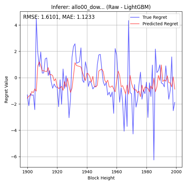
To gain some insight as to why the per-inferer z-score models perform best we compare the predicted and true values for each target variable, using the forecaster models with EMA=[3,7] and autocorrelation as an example. In the figures smaller loss, larger regret and larger z-score indicate better performance. The three outperforming workers (downtrending, uptrending, crabbing) are indicated in the legends (blue, orange and green points, respectively). As previously, unfilled squares show the medians and dashed lines show linear fits for each worker.

Global/combined models:

Per-inferer models:

In general, the per-inferer models show better differentiation between workers. The combined models tend to put all ‘bad’ (random) inferers on similar relations, but the per-inferer models can distinguish some differences between them. Similarly, the linear fits for the per-inferer models tend to be closer to the ideal 1:1 line; i.e. the per-inferer models are more context aware, being better able to predict out- or under-performance for each individual worker.

For the target variable, the loss forecaster has the most difficult task: it needs to try and predict the absolute performance of each worker, which can vary dramatically from epoch to epoch. The predicted losses then need to be converted to regrets (difference from the full network loss, i.e. a measure of the expected outperformance relative to the network inference) for the weighting calculation. This can be simplified by instead directly predicting regrets, which provides a more stable property to predict by removing systematic epoch-to-epoch variations in losses, and indeed regret forecasters tend to outperform the loss forecasters.

One potential issue with regrets, which can be seen above for the crabbing worker, is that if the network inference becomes close to the worker inference (i.e. the network has identified it as an outperforming worker) its regret will trend to zero and it will no longer clearly be recognised as outperforming. For this reason we considered the regret z-score (difference from the mean regret of all inferers, divided by the standard deviation) as an alternative prediction target, as it identifies outperformance relative to other workers. Dividing by the standard deviation allows performance to be normalised across different epochs, which can be seen in the more consistent minimum and maximum true values between different workers. As we find, these properties allows z-score forecasters to significantly outperform both the regret and loss forecasters for this test.

[joel]

Now we understand what forecasting models are likely to perform well and why, it is time to apply them to real data. For this we apply the same methodology as the previous experiment, but now for ETH/USD and BTC/USD 5min prediction topics. The testing here is off-chain, so the forecasters are not contributing to the network inferences.

The results here reflect what we already saw in the synthetic network experiment:

• Per-inferer models outperform global/combined models.
• Regret z-score provides the best target variable, with raw regrets the next best. Both outperform the naive network inference and the best inferer.
• Shorter EMA lengths generally outperform longer lengths.

However, there are also some differences between the real topics and the synthetic one:

• Raw regrets models are much closer in performance to the z-score models.
• Per-inferer models with loss as a target perform worse than the best inferer (both ETH and BTC topics) and the naive network inference (ETH topic).

ETH/USD 5min Prediction:

BTC: 5min Prediction:

Differences between the experiments suggest there may not be a single optimal model, but that it may depend on the situation. For this reason, we suggest a suite of per-inferer forecasters (each predicting losses, regrets and z-scores) may provide a better solution, so that the network can identify the best performing forecaster model for its case.