Although I haven’t yet evaluated the impact of individual log-return-derived features on the model, the following is a report on how applying a selected set of these features improves performance. I will continue this analysis and provide a detailed report on the effect of individual features soon.
I planned my research process as follows:
I downloaded two full years (730 days) of ETH price data from Tiingo at 5-minute intervals and modified the dataset as described here. The data was then split into two parts—validation and test sets—ensuring that each contained sufficient context for training.
I began by fitting a linear regression model using varying look-back windows—our “context lengths”—to identify the optimal amount of historical data for forecasting. Treating context length L as a hyperparameter, I evaluated each candidate value on the validation set. For a given L, the model was retrained on the most recent L observations and then used to predict the next batch of returns. Each batch comprised 288 consecutive five-minute bars (one trading day), after which the window advanced by 288 points and the process repeated. This moving-window scheme ensured that the model continuously learned from fresh data while allowing us to empirically select the context length that maximized out-of-sample performance.
I believe that this walk-forward approach to retraining—rather than training on a fixed dataset and making all subsequent predictions—enables the model to continually adapt to new and emerging patterns. This is particularly important when working with time-series data, where market behavior can shift over time.
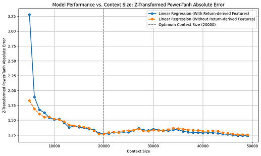
To determine the optimal context length, the model was retrained at each step using varying context sizes just before the test data. Three evaluation metrics were calculated across all batches (~6 months of validation data, totaling 50,000 prediction points) for each context length: directional accuracy (DA), relative absolute return-weighted RMSE improvement, and Z-transformed power tanh absolute error (ZPTAE). The results are as follows:
The optimal context length identified from this analysis was 20,000 (approximately 70 days), which yielded a directional accuracy (DA) of ~54.4%, a ZPTAE of 1.25, and a relative absolute return-weighted RMSE improvement of -25%.
Following this, I incorporated several log-return-based features into the dataset, including:
- Bollinger Bands: Upper and lower bands derived from the rolling mean and standard deviation of returns over a 48-hour window.
- Relative Strength Index (RSI): Calculated over 6-hour and 24-hour windows.
- Moving Average Convergence Divergence (MACD): Computed using default parameters from Python’s TA package.
- KST (Know Sure Thing): Also calculated with the default settings from Python’s TA package.
- Simple and Exponential Moving Averages (SMA & EMA): Derived from the return series over 6h, 12h, 24h, 48h, and 96h windows to capture various trend horizons.
- SMA Differences: Such as SMA(12h) − SMA(6h) and SMA(24h) − SMA(12h), to highlight momentum shifts.
- Exponentially Weighted Standard Deviation: Computed using smoothing factors α = 0.01 and 0.05.
- Trend Deviation: Defined as the difference between the 24-hour EMA of return and the current return.
Upon reevaluation with these features, the model’s directional accuracy improved noticeably across nearly all context lengths, while the relative RMSE improvement and ZPTAE loss remained largely unchanged.
It can be interpreted from the above plots that, when we extend the context window, both relative RMSE improvement and our custom ZPTAE metric rise steadily and then level off around the optimal look-back length, but DA doesn’t follow that pattern, and even declines with longer horizons. This suggests that DA on its own can be misleading, as you might correctly predict direction less than half the time yet still profit if your correct calls coincide with large market moves, a nuance that ZPTAE captures by scaling errors with volatility and return size. The drop in DA beyond the ideal window may also hint at overfitting to outdated patterns, whereas RMSE-based measures remain stable. Overall, this highlights the value of error metrics that weight by return magnitude, rather than relying solely on raw hit rates—especially when the model or its features aren’t yet strong enough to consistently make high-confidence directional predictions.
I then evaluated the model on the test set using three versions of the dataset: one without return-derived features, one with them, and one with return-derived features after applying feature reduction. The results below reflect the model’s performance when predicting log-returns over one year of test data—approximately 100,000 predictions—using a context length of 20,000 data points:
These results demonstrate that log-return-derived features significantly enhance the model’s performance, with feature reduction offering further improvements.
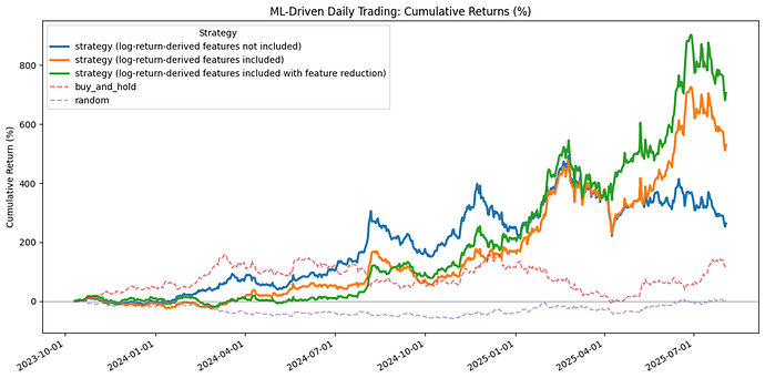
Finally, I trained the model on these datasets and simulated daily trading over a 2-year period, resulting in a total of 663 trades. The cumulative returns were as follows:
- 260% for the model without log-return-derived features,
- 530% with log-return-derived features, and
- 708% with log-return-derived features plus feature reduction.
For comparison, simply holding the asset yielded a return of 122%, while random trading resulted in a -1% return. These results demonstrate the promising potential of log-return-derived features in enhancing model performance and trading outcomes.


